An image encryption approach on the basis of the time delay chaotic system

【论文地址】

一种基于时滞混沌系统的图像加密方法

摘要

本文研究了基于时滞混沌系统的图像加密问题。首先提出了一种时滞混沌系统，该系统随时滞的变化具有不同的动力学行为。然后，根据新系统的时延，设计了一种新的图像加密方法。最后的实验表明，所提出的图像加密方法具有良好的有效性和较高的安全性。

引言

随着计算机网络的迅速发展，数字图像可以高速传输到世界的任何一个角落。然而，恶意用户也可以利用计算机网络获取未经授权的数字图像。因此，对这些未经授权的图像进行加密，防止图像信息被截获具有重要意义。

图像加密问题已经得到了深入而广泛的研究，提出新的图像加密机制是很有必要的。混沌图像加密技术提供了一种有效的解决方案，到目前为止，已经提出了许多混沌系统。在现实世界中，时延广泛存在，研究表明，时延的微小变化可以极大地改变混沌系统的动态行为，可以用来设计图像加密方案。然而，据我们所知，现有的时滞混沌系统数量较少，几乎没有利用混沌系统的时滞进行图像加密的研究。

新型时滞混沌系统

首先，提出了一种新的时滞混沌系统定义如下：

$$\left\{ \begin{array}{l} \frac{dx(t)}{dt}=a(y(t)-x(t))+w(t) \\ \frac{dy(t)}{dt}=(c-z(t))x(t)-y(t-\tau) \\ \frac{dz(t)}{dt}=x(t)y(t)-bz(t) \\ \frac{dw(t)}{dt}=-x(t)-aw(t) \end{array} \right .$$

其中，系统初始值(x0,y0,z0,w0)=(0.1,0.1,0.1,0.1) ,控制参数为a=1.5,b=0.5,c=10.6,$\tau$=6.5时系统的动力学行为表现如下图：

注：时滞混沌系统的时滞初始条件由定义在 $[-\tau,0]$上的 连续函数给出，论文中并没有说明？？？本文采用 $y0=sin(t),t\in [-\tau,0]$。

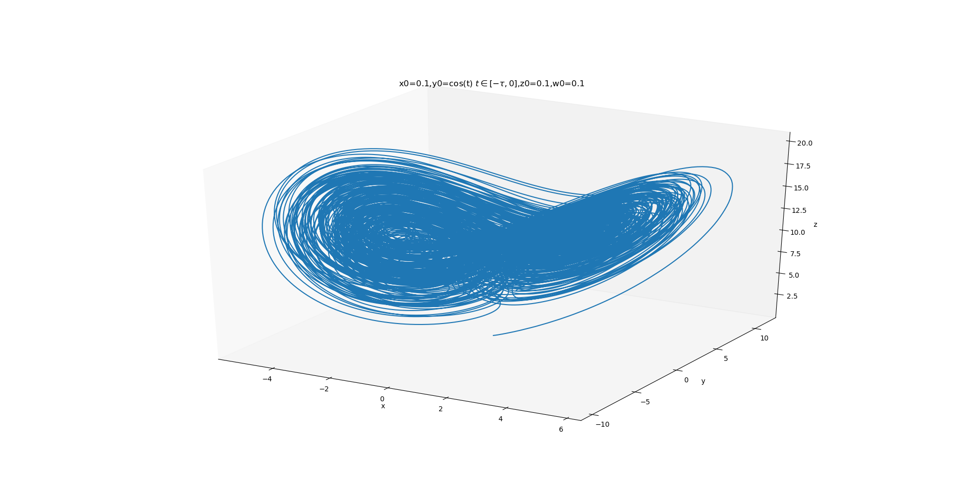
可以看出，所提出的时滞系统具有非常复杂的混沌动力学行为。

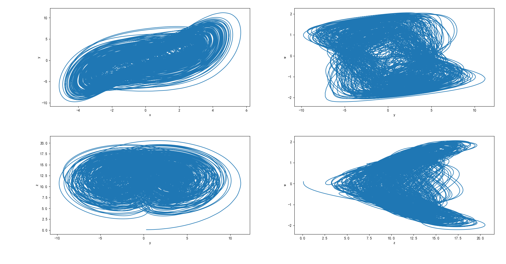
系统状态变量的相图如下：

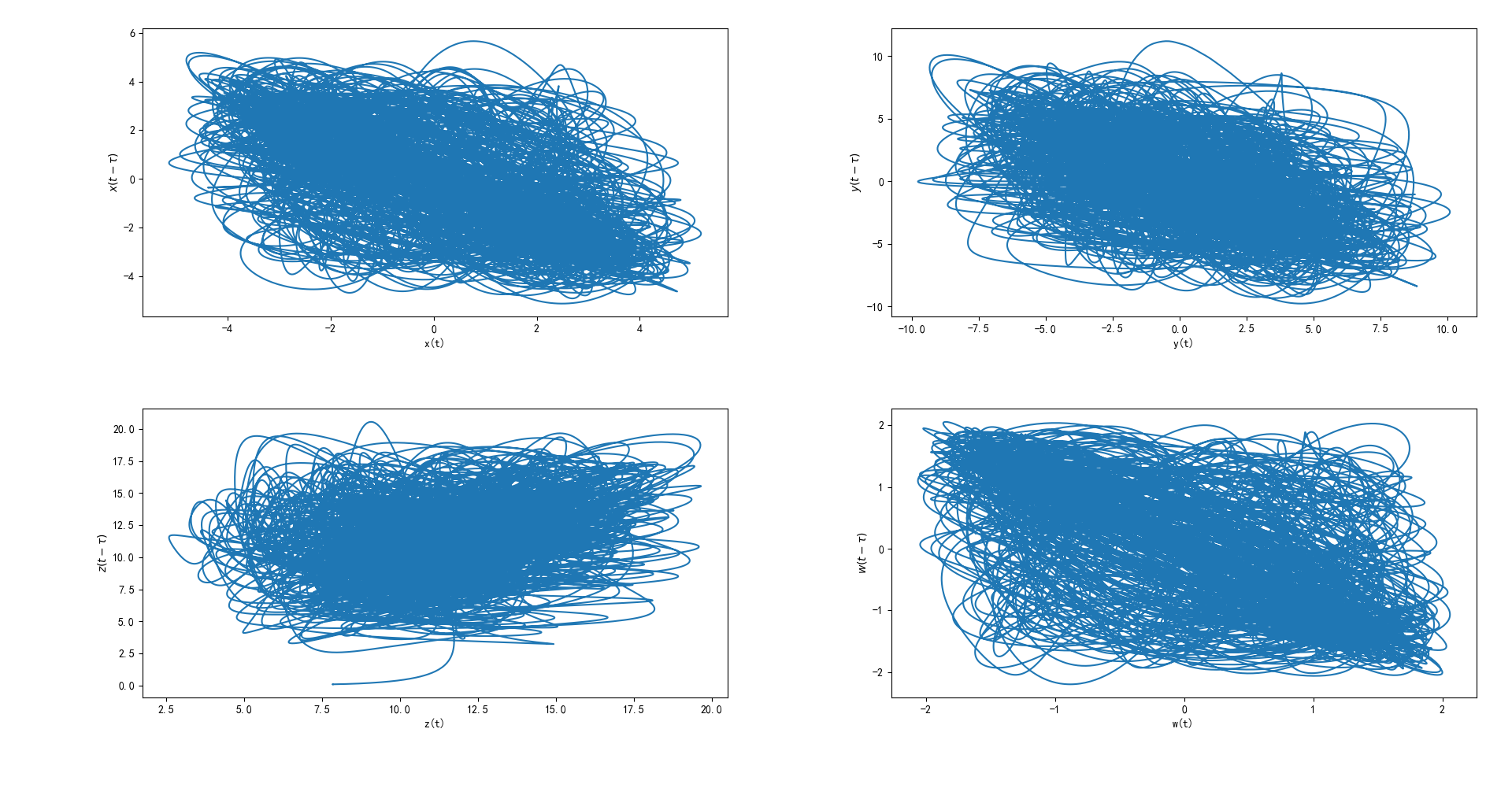
系统状态变量和延迟状态变量的相图如下：

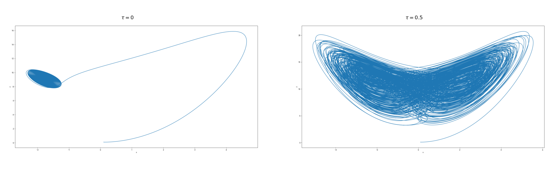
然后，考虑时滞对新系统动力学行为的的影响。当a=1.5,b=0.5,c=10.6,(x0,y0,z0,w0)=(0.1,0.1,0.1,0.1)时，给出了具有不同时滞的新系统的动力学行为如下：

注：同样，本文采用 $y0=sin(t),t\in[-\tau,0]$。

图像加密

论文里一堆公式，也没有文字描述，没啥好讲的，下面介绍本文实验采用的加密方式

步骤一

根据 $\tau_1=3.0,\tau_2=4.0,\tau_3=6.0$迭代生成三次不同的时滞混沌序列。每次从x(t),y(t),z(t),w(t)中都选择x(t)，最后得到三个长度为M*N*8(M*N为图像大小)的混沌序列。(这里可以改成利用一次迭代生成的四个序列中的三个，可以加快速度，提高效率)

步骤二

然后根据下面公式，把混沌序列转成01序列：

$$p^{l}(k)= \left\{ \begin{array}{l} 0,q^l_s(k)<v \\ 1,q^l_s(k)\geq v \end{array} \right .$$

其中，s=3,v=5,其中s表示小数点后第几位的值，v代表阈值。

步骤三

然后把三个01混沌序列，每八个作为二进制值转成一个0-255之间的值，得到3个大小为M*N的值为0-255之间的混沌序列 $U_{M*N}$ 。

步骤四

根据下式得到三个异或运算后的R、G、B通道

$$E_{M*N}=XOR(R_{M*N},U_{M*N})$$

步骤五

三通道合并得到加密图像，解密过程和加密过程相同。

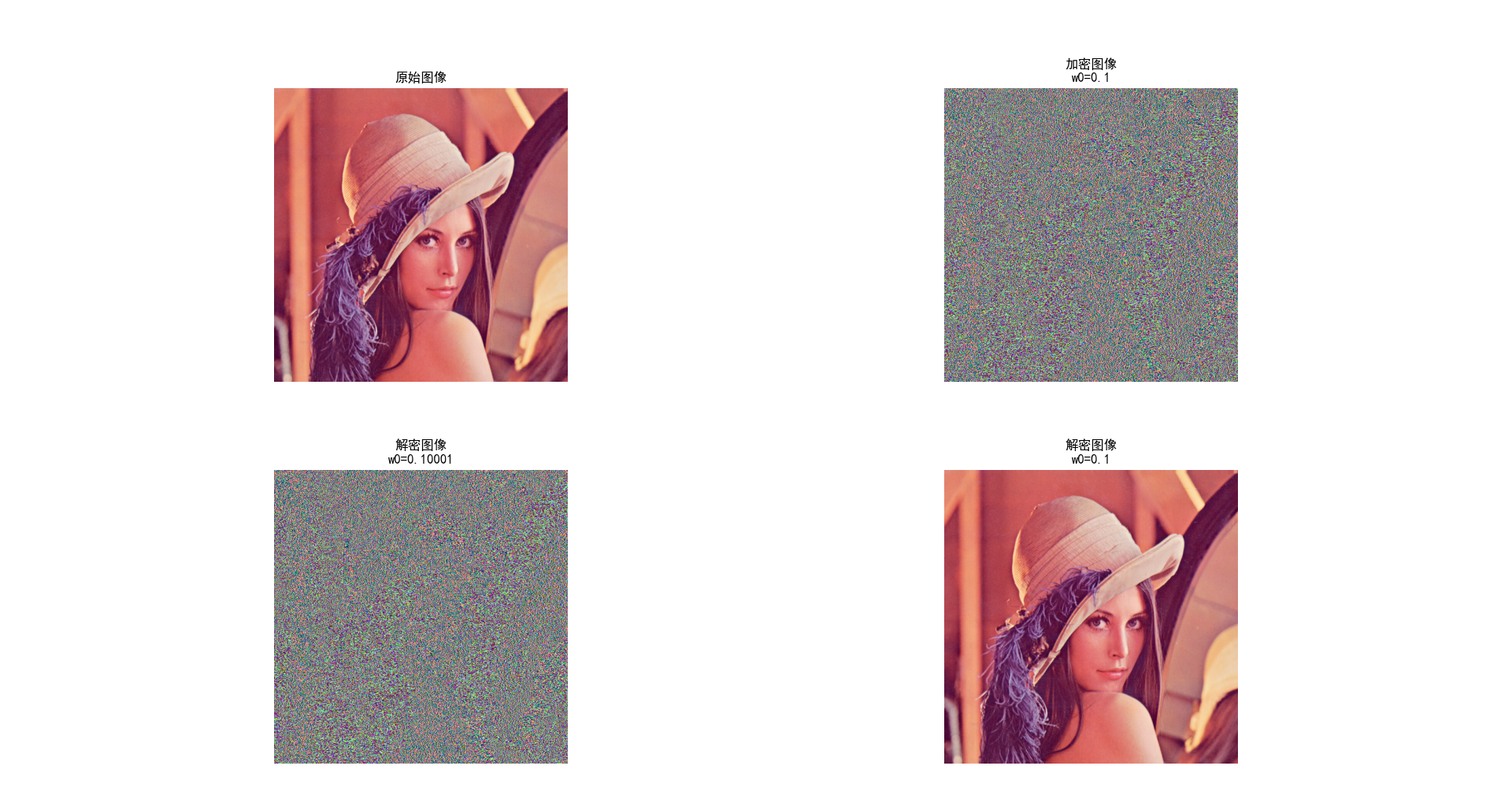
实验结果

实验代码

时滞混沌系统

import numpy as np
import matplotlib.pyplot as plt
#绘制三维图像
import mpl_toolkits.mplot3d as p3d


'''
新型时滞混沌系统吸引子生成函数
参数为4个初始坐标，4个初始参数(包含时滞参数）,迭代次数
返回4个一维数组（可以生成5个混沌序列）
初始条件的连续函数按y0处理
'''
def time_delay(h,x,y,z,w,a,b,c,tao,T):
  for t in range(T):
    x[t+1]=x[t]+h*(a*(y[t+tao]-x[t])+w[t])
    y[tao+t+1]=y[t+tao]+h*((c-z[t])*x[t]-y[t])
    z[t+1]=z[t]+h*(x[t]*y[t+tao]-b*z[t])
    w[t+1]=w[t]+h*(-x[t]-a*w[t])
  return x,y[tao:],z,w

def main():
  #设定参数
  a=1.5
  b=0.5
  c=10.6
  tao=6.5
  #迭代次数
  T=1000000
  #设初值
  x0=0.1
  y0=0.1
  z0=0.1
  w0=0.1
  # fig=plt.figure()
  # ax=p3d.Axes3D(fig)
  #迭代步长的设置很重要
  h=0.001
  tao=int(tao/h)
  #初始值加上迭代T次，最后的序列长度是T+1
  x=np.arange(x0,T+1,dtype=np.float64)
  y=np.arange(y0,T+tao+1,dtype=np.float64)
  z=np.arange(z0,T+1,dtype=np.float64)
  w=np.arange(w0,T+1,dtype=np.float64)
  #时滞y(t)在[-tao,0]内的初始函数
  for i in range(tao+1):
    y[i]=np.sin(i)
  #得到时滞混沌系统产生的序列，大小为T+1
  x,y,z,w=time_delay(h,x,y,z,w,a,b,c,tao,T)

  #结果展示
  plt.rcParams['font.sans-serif'] = ['SimHei']  # 中文乱码
  plt.rcParams['axes.unicode_minus']=False  #正确显示负号

  ##结果展示，系统吸引子
  ax=plt.subplot(111,projection="3d")
  ax.plot(x,y,z)
  ax.set_xlabel('x')
  ax.set_ylabel('y')
  ax.set_zlabel('z')
  ax.set_title('x0={0},y0=cos(t) $t\\in[-\\tau,0]$,z0={1},w0={2}'.format(x0,z0,w0))
  #消除网格
  ax.grid(False)
  #显示图像
  plt.show()

  #结果展示,系统状态变量相图
  plt.subplot(221)
  plt.plot(x,y)
  plt.xlabel('x')
  plt.ylabel('y')
  #不显示坐标轴
  # plt.axis('off')
  #子图2
  plt.subplot(222)
  plt.plot(y,w)
  plt.xlabel('y')
  plt.ylabel('w')
  plt.subplot(223)
  plt.plot(y,z)
  plt.xlabel('y')
  plt.ylabel('z')
  plt.subplot(224)
  plt.plot(z,w)
  plt.xlabel('z')
  plt.ylabel('w')
  # #设置子图默认的间距
  plt.tight_layout()
  #显示图像
  plt.show()

  #结果展示，系统状态变量和时延状态变量的相图
  plt.subplot(221)
  plt.plot(x[tao:],x[:T+1-tao])
  plt.xlabel('x(t)')
  plt.ylabel('$x(t-\\tau)$')
  plt.subplot(222)
  plt.plot(y[tao:],y[:T+1-tao])
  plt.xlabel('y(t)')
  plt.ylabel('$y(t-\\tau)$')
  plt.subplot(223)
  plt.plot(z[tao:],z[:T+1-tao])
  plt.xlabel('z(t)')
  plt.ylabel('$z(t-\\tau)$')
  plt.subplot(224)
  plt.plot(w[tao:],w[:T+1-tao])
  plt.xlabel('w(t)')
  plt.ylabel('$w(t-\\tau)$')
  # #设置子图默认的间距
  plt.tight_layout()
  plt.show()

  # #结果展示，不同时滞的相图
  # plt.subplot(111)
  # plt.plot(x,z)
  # plt.xlabel('x')
  # plt.ylabel('z')
  # # # #设置子图默认的间距
  # plt.tight_layout()
  # plt.show()

if __name__=='__main__':
  main()

图像加密解密

import cv2
import numpy as np
import matplotlib.pyplot as plt
#绘制三维图像
import mpl_toolkits.mplot3d as p3d


'''
新型时滞混沌系统吸引子生成函数
参数为4个初始坐标，4个初始参数(包含时滞参数）,迭代次数
返回4个一维数组（可以生成5个混沌序列）
初始条件的连续函数按y0处理
'''
def time_delay(h,x,y,z,w,a,b,c,tao,T):
  for t in range(T):
    x[t+1]=x[t]+h*(a*(y[t+tao]-x[t])+w[t])
    y[tao+t+1]=y[t+tao]+h*((c-z[t])*x[t]-y[t])
    z[t+1]=z[t]+h*(x[t]*y[t+tao]-b*z[t])
    w[t+1]=w[t]+h*(-x[t]-a*w[t])
  return x,y[tao:],z,w


def encrypt(img,key):
  im=cv2.imread(img)
  B,G,R=cv2.split(im)
  m,n,dim=im.shape

  #时滞混沌系统控制参数
  a=1.5
  b=0.5
  c=10.6
  tao0=key[0]
  x0=key[1]
  z0=key[2]
  w0=key[3]
  #迭代步长
  h=0.01
  #舍去前5000个暂态值
  T=m*n*8+5000
  seq=[]
  for tao in tao0:
    tao=int(tao/h)
    #初始值加上迭代T次，最后的序列长度是T+1
    x=np.arange(x0,T+1,dtype=np.float64)
    y=np.arange(0,T+tao+1,dtype=np.float64)
    z=np.arange(z0,T+1,dtype=np.float64)
    w=np.arange(w0,T+1,dtype=np.float64)
    #时滞y(t)在[-tao,0]内的初始函数
    for i in range(tao+1):
      y[i]=np.sin(i)
    #得到时滞混沌系统产生的序列，大小为T+1
    x,y,z,w=time_delay(h,x,y,z,w,a,b,c,tao,T)
    seq.append(x[5001:])
    seq.append(y[5001:])
    seq.append(z[5001:])
  for i in range(len(seq)):
    for j in range(len(seq[i])):
      seq[i][j]=0 if seq[i][j]*1000%10<5 else 1
    u=[]
    tmp=0
    for j in range(0,int(len(seq[i])/8)):
      tmp=seq[i][j]*2**7+seq[i][j+1]*2**6+seq[i][j+2]*2**5+seq[i][j+3]*2**4+seq[i][j+4]*2**3+seq[i][j+5]*2**2+seq[i][j+6]*2+seq[i][j+7]
      u.append(tmp)
    #强转类型为uint8，便于运算
    seq[i]=np.array(u).astype(np.uint8)

  #异或扩散
  #扁平化为一维
  R=R.flatten(order='C')
  G=G.flatten(order='C')
  B=B.flatten(order='C')

  R=R^seq[0]
  G=G^seq[1]
  B=B^seq[2]
  #转成二维
  R=R.reshape((m,n),order='C')
  G=G.reshape((m,n),order='C')
  B=B.reshape((m,n),order='C')
  #三通道合并
  encrypt=cv2.merge([R,G,B])
  return encrypt

'''
解密过程和加密过程完全一样
'''
def decrypt(img,key):
  return encrypt(img,key)

def main():
  #三个不同的tao值
  # tao0=[3.0,4.0,6.0]
  tao0=[3.0]
  #设初值
  x0=0.1
  z0=0.1
  w0=0.1
  key=[tao0,x0,z0,w0]

  img_path='./Lena.png'
  img=cv2.imread(img_path)[:,:,(2,1,0)]
  img_encrypt=encrypt(img_path,key)
  encrypt_path='./Lena_encrypt.png'
  cv2.imwrite(encrypt_path,img_encrypt[:,:,(2,1,0)])

  #正确密钥解密图像
  img_decrypt=decrypt(encrypt_path,key)
  decrypt_path='./Lena_decrypt.png'
  cv2.imwrite(decrypt_path,img_decrypt[:,:,(2,1,0)])

  #错误密钥解密图像
  wrong_key=list(key)
  wrong_key[3]+=pow(10,-5)
  wrong_decrypt=decrypt(encrypt_path,wrong_key)
  cv2.imwrite('./wrong_decrypt.png',wrong_decrypt[:,:,(2,1,0)])

  #结果展示
  plt.rcParams['font.sans-serif'] = ['SimHei']  # 中文乱码
  #子图1，原始图像
  plt.subplot(221)
  #imshow()对图像进行处理，画出图像，show()进行图像显示
  plt.imshow(img)
  plt.title('原始图像')
  #不显示坐标轴
  plt.axis('off')

  #子图2，加密后图像
  plt.subplot(222)
  plt.imshow(img_encrypt)
  plt.title('加密图像\nw0={}'.format(key[3]))
  plt.axis('off')

  #子图3，错误密钥解密结果
  plt.subplot(223)
  plt.imshow(wrong_decrypt)
  plt.title('解密图像\nw0={}'.format(wrong_key[3]))
  plt.axis('off')

  #子图4，正确密钥解密结果
  plt.subplot(224)
  plt.imshow(img_decrypt)
  plt.title('解密图像\nw0={}'.format(key[3]))
  plt.axis('off')

  # #设置子图默认的间距
  plt.tight_layout()
  #显示图像
  plt.show()

if __name__=='__main__':
  main()

疑问

时滞动力系统初始值？？？

对时滞动力系统，其初始条件为连续函数，论文中并没有提到初始条件的连续函数，不知道是怎么处理的，一律按0处理？？？

混沌系统求解？？？

龙格库塔求解，欧拉公式求解

彩色？灰度？

论文里实验用的灰度图片？？？

密钥？？？

论文中并没有明确给出密钥空间的构成，x0,y0,z0,w0？？？

扩展

相图

广义相图是在给定条件下体系中各相之间建立平衡后热力学变量强度变量的轨迹的集合表达，相图表达的是平衡态，严格说是相平衡图。

总结

哇，这篇论文写得真是服了，依鄙人愚见，这篇论文真的不太ok，我觉得论文里还是存在很多问题的，要么是技术问题，要么是语言表达问题，记录如下：

我觉得论文最大的问题就是缺少文字描述，开篇引言还算行吧。。然后混沌系统就给了一个公式，然后就是插图。。。之后又是一堆算法公式，最后就是实验结果图片了。What？？？这也能发论文？？？

首先，时滞混沌系统都没讲明白，初值缺少连续函数。。不知道论文中混沌图像实验是怎么得来的。然后是加密算法，前面一堆公式就是为了生成混沌序列，公式也没有详细的说明，也不知道有什么理论依据，最后用了一个简单的异或操作进行图像加密。。。

当然，因为我还是刚刚入门图像加密领域，上述分析仅仅是根据本人所知得到的结论，不排除是因为自己太菜没看懂论文😗。

要不是花了两天时间在看时滞混沌系统，真的都不想实现这篇论文了，最后我还是简单地实现了一下，当做练手吧，以后看论文要看好论文，发表期刊影响因子大于3甚至4以上，不然要是因为论文问题耽误时间甚至是误导学习就得不偿失了。。

参考

【时滞混沌系统】

【相图】